


Madly Mapping the Universe
Software Make Spectacular Images of the Infrared Cosmos
February 3, 2010
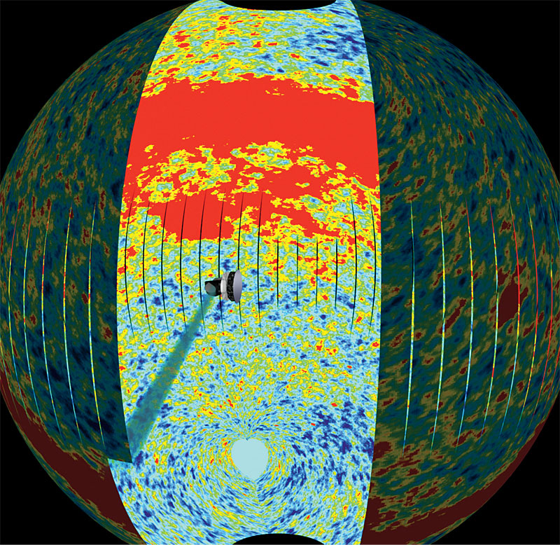
The MADmap code produces sky maps from the kind of data produced by cosmic microwave background (CMB) experiments like the Planck satellite (center). Written with large data sets in mind, MADmap works well on any time-ordered data set with “colored” noise. (Image credit European Space Agency)
To map our home planet, Google Earth depends mostly on satellite imagery for land surfaces and sonar imagery for the sea floor. Maps of the Universe likewise depend on different kinds of detectors for different kinds of features. Maps of the cosmic microwave background (CMB), for example, depend on measuring minute differences in the temperature of the sky.
When astrophysicist Julian Borrill came to Berkeley Lab’s National Energy Research Scientific Computing Center (NERSC) in 1997, his first project was designing computational tools for future CMB experiments, a toolbox capable of handling an expected flood of cosmic data. He and his colleagues Radek Stompor and Andrew Jaffe devised the Microwave Anisotropy Dataset Computational Analysis Package, or MADCAP. An essential part of the kit was a module for making maps.
Signal Versus Noise
Mapping the CMB requires accurately accounting for noise in the data. Each pixel begins as part noise and part signal. “White” noise has the property that each measurement is independent of all the others and can accurately be averaged, so it’s easy to account for the noise and estimate the signal’s contribution to the mix.
“Colored” or correlated noise is more challenging: here pixel noise varies across the sky, and its values are interrelated according to the particular path that the telescope has scanned during an exposure.
“You can’t account for correlated noise by just averaging it,” says Borrill, now with the Computational Cosmology Center (C3) in Berkeley Lab’s Computational Research Division. “To make a map it takes a special code to weigh and account for the noise in each pixel at each point in time.”
The detectors used to measure the temperature of the cosmic microwave background are particularly susceptible to colored noise, so the MADCAP bundle of codes included one specially designed to make maps from data where the noise is not white. Programmed by C3 member Christopher Cantalupo, the code is named MADmap.
The best detectors for measuring radiation at wavelengths between a millimeter and a fifth of a millimeter, where much of the CMB radiation lies, are bolometers. (CMB radiation at lower frequencies is measured with radiometers.) A bolometer gauges how much an incoming photon heats up a very cold detector, whose temperature is kept at a tiny fraction of a degree above zero degrees Kelvin. Correlated or colored noise is a known characteristic of bolometers.
“Because a bolometer’s temperature can never be at absolute zero, it will always have some thermal noise,” Borrill says. This noise level varies as the bolometer’s temperature changes. “Another source of noise is that when a photon hits a bolometer, it ‘rings’ for a while.”
As for the first kind of noise, Cantalupo says, “because the refrigerator is not perfect there are long-term drifts in temperature; the noise changes slowly with time.”
He compares the colored-noise problem to the situation of a traffic patrolman using a radar gun to determine the expected speed of passing cars. “If there is very little traffic, the speed of one car will be largely independent of the speed of the others. But if the traffic becomes dense, cars traveling near each other are likely to be traveling at similar speeds,” he explains. “There will still be some variation in speed, and this scatter in the measurements is colored noise.”
To determine the expected speed of a passing car based on the speeds of cars previously measured, the correlation among cars when traffic is dense must be taken into account – especially the noise of the scatter of measurements in heavy traffic – so that these measurements are not given too much significance in the final estimate.

When used to decode data from the bolometers in the PACS instrument aboard the Herschel satellite (left), MADmap yields images like this 2 x 2 degree area of the sky in the constellation of the Southern Cross.
“If we give more significance to measurements taken farther apart in time, we can make a better estimate of the underlying signal,” Cantalupo says.
Cantalupo describes the MADmap process as first collecting the basic data, a widely varying curve with fine structure imposed on large excursions, including information on where the instrument is pointed in the sky and the time during which the data was collected. The data is filtered to remove “average” noise — “but of course we haven’t just filtered noise but signal too,” says Cantalupo.
The math that determines how the noise is correlated from time to time within each pixel is performed on this smoothed-out, filtered data. Then the filtering is undone to restore the signal – which for CMB data is the emperature of the sky for each pixel in the map.
MADmap Spreads Its Wings
Borrill says that although MADmap was designed with CMB data in mind, “it was always intended to be independent of the specifics of any one experiment.”
MADmap has been used for CMB experiments from the balloon-borne MAXIMA, which mapped a portion of the northern sky in 1998, and BOOMERANG, which circled the South Pole in 1999, on up to the European Space Agency’s Planck satellite, launched on an Ariane rocket from French Guiana in May 2009; all these experiments and others record data in different formats, so MADmap’s flexibility is essential.
MADmap is so flexible, in fact, that it is applicable to any kind of experiment whose data is similar to the model it was built for. From the beginning, it has been posted on the Internet as open-source software.
Enter Herschel, a satellite that by coincidence was launched on the same Ariane rocket as Planck. Unlike Planck, Herschel is an infrared observatory. It carries a 3.5-meter telescope, the most powerful infrared telescope ever flown in space. The principal detectors for one of its three instruments, the Photoconductor Array Camera and Spectrometer (PACS), are two arrays of highly sensitive bolometers. In 2007, long before Herschel and Planck were launched, Cantalupo got a call from Pierre Chanial, a PACS scientist who was developing the instrument’s mapping software.
“He wanted know if it was okay with us if he used MADmap as the core map-making software for PACS,” Cantalupo says. “He said it was suggested to him by Andrew Jaffe, who had designed the original MADCAP with Julian.”

From top, Julian Borrill, Christopher Cantalupo, and Ted Kisner
Cantalupo and Borrill and their colleagues were delighted that MADmap promised to be useful in unanticipated ways. The PACS bolometers are photometers designed to collect far-infrared light, mapping galaxies and other objects whose internal structures are obscured, such as clouds of gas and dust where new stars are being born or disks in which solar systems may be forming. But the novel application of MADmap to the infrared data introduced some challenges.
“The PACS data-transfer pipeline needs to use Java, which had not been contemplated when MADmap was written,” Cantalupo says. “So we were able to be of some use in helping with the rewrite.”
Different questions arose when Herschel began making images in July after reaching orbit at Lagrangian Point 2, where the combined gravity of Earth and Sun maintain the satellite mostly in the Earth’s shadow — thus an excellent place for an observatory. C3’s Theodore Kisner became involved in the effort to help the PACS team make the best of MADmap.
“There was some trouble with the real data relating to the character of the noise,” Kisner says. “Since I’ve been working with noise estimation, I was able to contribute to this aspect.”
The way PACS makes an image is different from the way a CMB instrument maps the sky: a CMB experiment essentially scans across the sky in one smooth stroke after another, whereas, Kisner says, “Herschel kind of wobbles around, looking at the same region sort of like looking through a hole in a fence.”
Noise estimation is easier for Herschel in some ways, not only because its bolometers are very stable but because they map specific regions; unlike the ubiquitous cosmic microwave background, “parts of the sky in a Herschel image are actually dark,” Kisner says. “No signal at all is a perfect baseline for accounting for noise.”
Nevertheless, what the two kinds of observations have in common is that both depend on time-streams of data, which is where correlated noise resides.
“Our major hope now is that we can persuade the PACS folks away from using Java and instead toward using our latest version of MADmap,” Cantalupo says. “Some of their observations require very long exposures, where our new Version 2 will be very helpful. On the smaller observations, the Java version is okay.”
Already the C3 team has devised a new secondary format for Herschel that will be able to handle various kinds of data. MADmap 2 readily reads data in different formats and would be easier to use and more flexible that the present version.
“It’s completely their decision,” says Cantalupo. “We’re just happy to be useful.” He and Kisner have attended data processing workshops at the NASA Herschel Science Center at Caltech to show scientists who are using Herschel good ways of using MADmap.
For his part, Julian Borrill is delighted that a program initially developed with support from NASA’s Applied Information Systems Research program and Berkeley Lab’s Laboratory Directed Research and Development program has spread its wings and has already proved its merit for analyzing very different kinds of astronomical data.
Learn More
»Tackling CMB data with MADCAP
» Wikipedia’s article on bolometers
» The launch of Planck (and Herschel)
About Berkeley Lab
Founded in 1931 on the belief that the biggest scientific challenges are best addressed by teams, Lawrence Berkeley National Laboratory and its scientists have been recognized with 16 Nobel Prizes. Today, Berkeley Lab researchers develop sustainable energy and environmental solutions, create useful new materials, advance the frontiers of computing, and probe the mysteries of life, matter, and the universe. Scientists from around the world rely on the Lab’s facilities for their own discovery science. Berkeley Lab is a multiprogram national laboratory, managed by the University of California for the U.S. Department of Energy’s Office of Science.
DOE’s Office of Science is the single largest supporter of basic research in the physical sciences in the United States, and is working to address some of the most pressing challenges of our time. For more information, please visit energy.gov/science.