Introduction

The Roofline model is oriented around the interplay between application data locality, data bandwidth, and computational throughput.  Each of these topics are further refined and discussed here.

Arithmetic Intensity

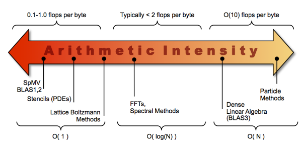
The core parameter behind the Roofline model is Arithmetic Intensity. Arithmetic Intensity is the ratio of total floating-point operations to total data movement (bytes). A BLAS-1 vector-vector increment ( x[i]+=y[i] ) would have a very low arithmetic intensity of 0.0417 (N FLOPS / 24N Bytes) and would be independent of the vector size. Conversely, FFT's perform 5*N*logN flops for a N-point double complex transform. If out of place on a write allocate cache architecture, the transform would move at least 48N bytes. As such, FFT's would have an arithmetic intensity of 0.104*logN and would grow slowly with data size. Unfortunately, cache capacities would limit FFT arithmetic intensity to perhaps 2 flops per byte. Finally, BLAS3 and N-Body Particle-Particle methods would have arithmetic intensity grow very quickly.

Roofline Model

The most basic Roofline model can be used to bound Floating-point performance as a function of machine peak performance, machine peak bandwidth, and arithmetic intensity.

One can visualize the Roofline model by plotting the performance bound (GFlop/s) as a function of Arithmetic Intensity. The resultant curve can be viewed as a performance envelope under which kernel or application performance exists.

Effects of NUMA on Memory Bandwidth

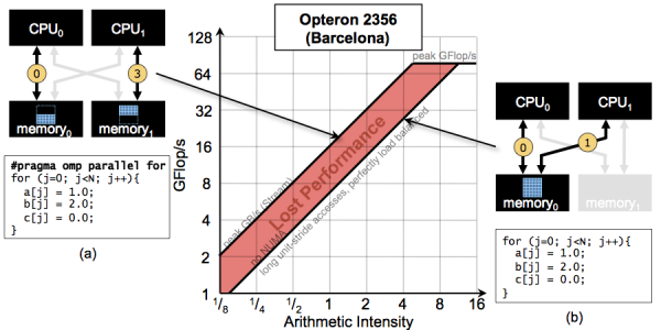
Modern SMPs and GPU-accelerated systems will present non-uniform memory access. Depending on the locality of data and the placement of threads, memory bandwidth can vary dramatically. The following example highlights the impact of first-touch allocation of data in OpenMP on bandwidth. In effect, the resultant lower bandwidth can depress performance for virtually any attainable arithmetic intensity.  

Effects of Cache Behavior on Arithmetic Intensity

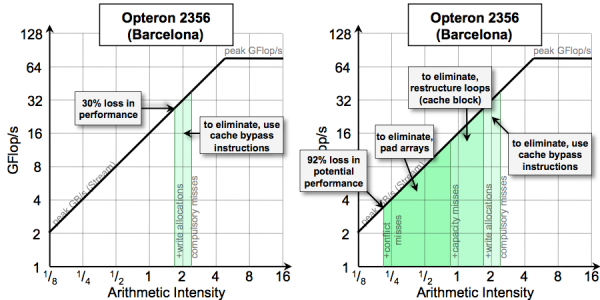
The Roofline model requires an estimate of total data movement. On cache-based architectures, the 3C's cache model highlights the fact that there can be more than simply compulsory data movement. Cache capacity and conflict misses can increase data movement and reduce arithmetic intensity. Similarly, superfluous cache write-allocations can result in a doubling of data movement. The vector initialization operation x[i]=0.0 demands one write allocate and one write back per cache line touched. The write allocate is superfluous as all elements of that cache line are to be overwritten. Unfortunately, the presence of hardware stream prefetchers can make it very difficult to quantify how much beyond compulsory data movement actually occurred.

Instruction-Level Parallelism and Performance

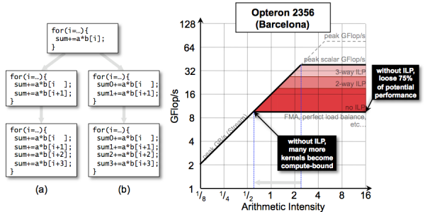
Modern processor architectures are deeply pipelined. Although this can increase frequency and peak performance, it does increase the latency of various instructions. In order to avoid bubbles in the pipeline and attain peak performance, the programmer and compiler must collaborate and ensure independent instructions are issued in sequence (instruction-level parallelism). A lack of ILP can depress performance on sufficiently compute-intensive kernels. Conversely, on memory-intensive operations, a lack of ILP may not impede performance. The example below highlights this in a contrived summation example in which partial sums are constructed and summed at the conclusion of the loop.  

Data-Level Parallelism and Performance

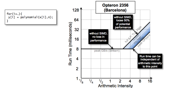
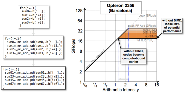
Data-level parallelism (vectorization, SIMDization, etc...) has become a very attractive approach to maximizing performance and energy efficiency. Unfortunately, attainable performance is highly dependent on the compiler or programmer's ability to exploit these instructions. For high arithmetic intensity, a lack of efficient SIMDization can depress performance. However, for low arithmetic intensities, the impact on performance may be negligible.  

Run Time vs Arithmetic Intensity

Rather than viewing Roofline as performance as a function of arithmetic intensity, one can use the model to understand the relationship between run time and arithmetic intensity. To do so, one must use the data set sizes convert performance (per element) into run time for all elements. In the example below, we show that run time is independent of the degree of the polynomial until one reaches the machine balance. Beyond that point, time to solution should increase linearly with the degree of the polynomial. Researchers should view this as an opportunity. One can change the algorithm (e.g., move to a high-order method and attain better error) without affecting run time.